PopJSON
We propose a JavaScript Object Notation (JSON) representation, named
PopJSON, for communicating and storing population dynamics models.
Ornamented with custom tags and operations, PopJSON describes the
essentials of a dynamically-structured multi-process matrix population
model. PopJSON is primarily designed to handle the sPop
models of Erguler et
al. [sPop,
sPop2,
Population],
but recent versions can also parse simple ODE models and even embed one
within another!
PopJSON requires a parser to translate it into code that can either be directly interpreted or compiled into an executable. For the Population package, the output should be raw ANSI C, however, many other canonical models can be parsed into R, Python, or any other scientific programming language.
In this repository, we included a
wrapper
to read and simulate the translated models into Python.
Soon, we will write another one for R.
We use the curly brackets {} throughout the text to group related tags and square brackets [] to define processess with a strict order. We hope all will be clearer as you read along.
Model definition
We define a Population model using the model tag, where the key fields are type and parameters. The system’s dynamics can be specified as either deterministic or stochastic via the boolean deterministic tag. If finer control is required, the istep tag can be used to set the precision of the accumulative process indicator (specific to the Population package), effectively limiting the maximum number of pseudo-stage classes.
Before following the steps below, we recommend having a look at the Population package description.
{
    "model": {
            "title": "Climate-sensitive population dynamics of Aedes albopictus",
            "type": "Population",
            "url": "https://github.com/kerguler/Population",
            "deterministic": true,
            "parameters": {
                "algorithm": "Population",
                "istep": 0.01
            }
        }
}
Declaring a population (or a development stage)
A population, by definition, is a structured collection of similar individuals. There exists classes in a population that are invisible to the end user, but they distinguish individuals into sub-groups. For example, an age-structured population of larvae is composed of individuals all at their larva stage of development, however, some have been there for long but some have just started. The time they turn into pupae depends on how long they have been in the stage.
{
    "populations": [
        {
            "id": "larva",
            "name": "The larva stage",
            "processes": [
                {
                    "id": "larva_dev",
                    "name": "Larva development time",
                    "arbiter": "AGE_GAMMA",
                    "value": [10, 4]
                }
            ]
        }
    ]
}
See ex1a.json and ex1a.c for full PopJSON representation and C translation. Use plot_ex1.py to run the model.
The above example represents a larva population with a development time of 10 days (with a standard deviation of 4 days). The population is age-structured and the development time is gamma-distributed.
Here, AGE_GAMMA refers to a specific population structure and development time distribution listed in this table. Accordingly, AGE_GAMMA takes two parameters, the mean and standard deviation of development. In the above PopJSON representation, these are given as the first and second elements of the list value.


Dependence on environmental variables
Development is strongly dependent on temperature in many insect species. We have demonstrated that accumulative processes are suitable representations for development under variable environments (Erguler et al. 2022). So, we will switch to ACC_ERLANG as the accumulative equivalent of the gamma-distributed age-structured development.
{
    "populations": [
        {
            "id": "larva",
            "name": "The larva stage",
            "processes": [
                {
                    "id": "larva_dev",
                    "name": "Larva development time",
                    "arbiter": "ACC_ERLANG",
                    "value": ["d2m", "d2s"]
                }
            ]
        }
    ]
}
Please note that we declared the mean and standard deviation of development in terms of two variables, d2m and d2s, which we will define shortly.
Next, we define an environmental variable, temperature, to feed into our model.
{
    "environ": [
        {
            "id": "temp",
            "name": "Temperature of the breeding pool (in °C)",
            "url": ""
        }
    ]
}
What we need now is a function to transform temperature into the mean and standard deviation of development (to define d2m and d2s).
{
    "functions": {
        "briere1": ["define", ["T","B","E","a"], ["?",["<=","T","B"],"365.0", ["?",[">=","T","E"],"365.0", ["min","365.0",["max","1.0", ["/","1.0",["exp", ["+","a",["log","T"],["log",["-","T","B"]],["*","0.5",["log",["-","E","T"]]]]]]]]]]],
    }
}
Please note that the function definition begins with define, which is a key word (an operator). The second in the list is the list of parameters (only a single letter for each), and the last is the equation. The mathematical equation notation were inspired from the MathJSON representation of CortexJS. The list of all operators can be found here.
This is the reciprocal of the Briere-1 function commonly used in ecological modelling.briere1(T,a,L,R) = e−{a+ln(T)+ln(T−L)+0.5ln(R−T)}
The function returns a large value (365 days of development) outside
of L and R and stays within 1 and 365
for all T. Please note that the accumulative
development algorithm in Population currently cannot handle
mean process time smaller than a unit.
The Briere-1 function translates into the following C code:
double dmin(double a, double b) { return a < b ? a : b; }
double dmax(double a, double b) { return a > b ? a : b; }

#define briere1(T,a,L,R) ((((T) <= (L))) ? (365.0) : ((((T) >= (R))) ? (365.0) : (dmin(365.0, dmax(1.0, (1.0 / exp(((a) + log((T)) + log(((T) - (L))) + (0.5 * log(((R) - (T))))))))))))
Next, we connect temperature with d2m and d2s using the intermediates tag. A key feature of this tag is that it computes first at the beginning of each iteration.
{
    "intermediates": [
        {
            "id": "d2m",
            "value": ["briere1", ["temp","TIME_1"], "d2m_a", "d2m_b", "d2m_c"]
        }, {
            "id": "d2s",
            "value": ["*", "d2s_c", "d2m"]
        }
    ]
}
Here, temp (temperature) is used as an operator to extract its TIME_1th element. TIME_1 refers to the previous time point (we used yesterday’s conditions to estimate today’s population).
Lastly, we define the parameters of the model to complete the temperature dependency of development time. For each, we declare an id, a value, and weather the parameter is fixed (constant:true) or user-defined (constant:false). Minimum an maximum values can also be defined using min and max tags, which could be useful when performing optimisation.
{
    "parameters": [
        {
            "id": "d2m_a",
            "constant": false,
            "name": "Larva development mean (a)",
            "value": -15
        }, {
            "id": "d2m_b",
            "constant": false,
            "name": "Larva development mean (b)",
            "value": 10
        }, {
            "id": "d2m_c",
            "constant": false,
            "name": "Larva development mean (c)",
            "value": 35
        }, {
            "id": "d2s_c",
            "constant": false,
            "name": "Larva development stdev (c)",
            "value": 0.2
        }
    ]
}
See ex1E.json and ex1E.c for full PopJSON representation and C translation. Use plot_ex1E.py to run the model.


Declaring multiple processes
The Population algorithm enables declaring multiple
processes on a population. For instance, we could define lifetime and
development time together having independent Erlang-distributed
durations. Strictly, they would not be completely independent as the
processes take place in the order they are defined. This means if we
define development before larva mortality, pupae could be produced under
conditions not suitable for larva survival. We do not want that.
Here, we define the two processes for larva (in the plausible order) and follow the dynamics.
{
    "populations": [
        {
            "id": "larva",
            "name": "The larva stage",
            "processes": [
                {
                    "id": "larva_mort",
                    "name": "Larva lifetime",
                    "arbiter": "ACC_ERLANG",
                    "value": [7, 2]
                },
                {
                    "id": "larva_dev",
                    "name": "Larva development time",
                    "arbiter": "ACC_ERLANG",
                    "value": [10, 4]
                }
            ]
        }
    ],
    "transformations": [
        {
            "id": "larva_death",
            "name": "Larva dying today",
            "value": "larva_mort"
        }, {
            "id": "larva_to_pupa",
            "name": "Larva developing into pupa",
            "value": "larva_dev"
        }
    ]
}
See ex2a.json and ex2a.c for full PopJSON representation and C translation. Use plot_ex2.py to run the model.
The following transformations tag is needed to bind larva_mort to larva_death and larva_dev to larva_to_pupa to make them visible (remember that internal population structure is hidden by default). Otherwise, only the size of the larva population is monitored.
{
    "transformations": [
        {
            "id": "larva_death",
            "name": "Larva dying today",
            "value": "larva_mort"
        }, {
            "id": "larva_to_pupa",
            "name": "Larva developing into pupa",
            "value": "larva_dev"
        }
    ]
}
The resulting larva population size and the number of larvae completing each process (mortality or pupa production) is given below.

Declaring initial conditions
Since version 1.2.19, the initial conditions, or an initial population configuration, can be declared using the init statement within a population declaration.
Here, we demonstrate this by extending the previous example as the following:
{
    "populations": [
        {
            "id": "larva",
            "name": "The larva stage",
            "processes": [
                {
                    "id": "larva_mort",
                    "name": "Larva lifetime",
                    "arbiter": "ACC_ERLANG",
                    "value": [7, 2]
                },
                {
                    "id": "larva_dev",
                    "name": "Larva development time",
                    "arbiter": "ACC_ERLANG",
                    "value": [10, 4]
                }
            ],
            "init": [
                [0,0,100],
                [0,0.5,100]
            ]
        }
    ]
}
See ex2b.json and ex2b.c for full PopJSON representation and C translation. Use plot_ex2.py to run the model.
The two triplets, [0,0,100] and [0,0.5,100], add two population sub-groups, one with 100 individuals with 0 age counter and 0 development counter and the other one with 100 individuals with 0 age counter and 0.5 development counter. The latter corresponds to about 5 days of pre-development, half of the mean, which will result in an early production of pupae as shown in the figure below.

Simulating ODEs
As of version 1.6.0, PopJSON also supports the representation of ODE models. To illustrate this, we use the classic Lorenz chaotic system as an example.
To begin, set type: "ODE". This is an early
implementation, so for now models should remain deterministic (SDE
support will be added later) and time-independent (DDE support is
planned), and should use the rk8pd integration algorithm.
Basic solver options, such as the initial step size, and the absolute
and relative tolerances, can be specified.
{
    "model": {
        "title": "Lorenz equations",
        "type": "ODE",
        "deterministic": true,
        "parameters": {
            "algorithm": "rk8pd",
            "hstart": 1e-3,
            "eps_abs": 1e-8,
            "eps_rel": 1e-8
        }
    }
}
We set three populations and four parameters:
{
    "parameters": [
        {
            "id": "sigma",
            "constant": false,
            "value": 10.0
        }, {
            "id": "rho",
            "constant": false,
            "value": 28.0
        }, {
            "id": "beta",
            "constant": false,
            "value": 2.6666666666666665
        },{
            "id": "time_scale",
            "constant": false,
            "value": 1.0
        }
    ],
    "populations": [
        {
            "id": "xx"
        },{
            "id": "yy"
        },{
            "id": "zz"
        }
    ]
}
The time_scale parameter is critical. Although the ODE
system evolves in continuous time, outputs are recorded at discrete
integer steps. As a result, substantial dynamics may occur within a
single step - captured by the integrator but not directly visible in the
output. If this becomes an issue, you can effectively slow down the
system by adjusting time_scale.
Also, using x, y, and z as
population names may lead to namespace conflicts. If you specifically
need to use x as a population name, let me know and I can
look into resolving this.
The ODE system is represented as a Petri net, defined by a list of
reactions. The from and
to fields encode the stoichiometry of each reaction.
For example, "from": {"xx": 1} indicates that one unit of
xx is consumed by that reaction.
Here is the full Petri net:
{
        "reactions": [
        {
            "id": "r0",
            "to": { "xx": 1 },
            "value": ["*", "time_scale", "sigma", "yy"]
        },{
            "id": "r1",
            "from": { "xx": 1 },
            "value": ["*", "time_scale", "sigma", "xx"]
        },{
            "id": "r2",
            "to": { "yy": 1 },
            "value": ["*", "time_scale", "rho", "xx"]
        },{
            "id": "r3",
            "from": { "yy": 1 },
            "value": ["*", "time_scale", "xx", "zz"]
        },{
            "id": "r4",
            "from": { "yy": 1 },
            "value": ["*", "time_scale", "yy"]
        },{
            "id": "r5",
            "to": { "zz": 1 },
            "value": ["*", "time_scale", "xx", "yy"]
        },{
            "id": "r6",
            "from": { "zz": 1 },
            "value": ["*", "time_scale", "beta", "zz"]
        }
    ]
}
See ex8.json and ex8.c for full PopJSON representation and C translation. Use plot_ex8.py to run the model.
And, here is the result: 
Advanced usage
We can do more with the Populations package, and here we
describe a few interesting examples we could think of. Please
contact
us with requests or your own examples. Feel free to use the SandBox below.
Conditional transformations
We can include an if statement to conditionally execute any transformations, transfers, or migrations (see Declaring cyclic development and Vector dispersion modelling for more information on the latter two).
As an example, let’s use the if statement to delay introducing the population in the first example. Also, instead of introducing a naive cohort, let’s use the key statement to start with a population that has already experienced 5 iterations of development.
{
    "transformations": [
        {
            "id": "initial_structure",
            "to": "larva",
            "value": 100,
            "key": [5],
            "if": ["==", "TIME", 15]
        }
    ]
}
See ex1c.json and ex1c.c for full PopJSON representation and C translation. Use plot_ex1.py to run the model.
The “initial_structure” used above instructs the introduction of 100 larvae (with development indicator 5) into the population at time 15. As a result, the larvae will continue development for another 5 days and complete at time 20.

Declaring cyclic development (gonotrophic cycle)
Gonotrophic cycle is a complex process. After blood feeding, females develop eggs in their bodies and lay them before searching for blood again. To model the process, we define adult lifetime (adult_mort) and egg development (inside females) (adult_dev) for adult females.
{
    "populations": [
        {
            "id": "adult",
            "name": "Adult females",
            "processes": [
                {
                    "id": "adult_mort",
                    "name": "Adult lifetime",
                    "arbiter": "ACC_ERLANG",
                    "value": [20, 5]
                },
                {
                    "id": "adult_dev",
                    "name": "Egg development in adult females",
                    "arbiter": "ACC_ERLANG",
                    "value": [5, 1]
                }
            ]
        }
    ],
    "transformations": [
        {
            "id": "adult_death",
            "name": "Adult females dying today",
            "value": "adult_mort"
        }, {
            "id": "num_gravid",
            "name": "Number of gravid females",
            "value": "adult_dev"
        },{
            "id": "egg_laying",
            "name": "Egg laying at the end of gonotrophic cycle",
            "value": ["*", "num_gravid", 10]
        }
    ]
}
When adult_dev is completed (in 5 days plus or minus 1), we will have the females ready for egg laying. Then, the number of eggs laid can be estimated by employing an average, for instance, 10 eggs per gravid female (as in egg_laying).
The problem, however, is the need to add the females back into the population. For this, we define a transfer tag, which transfers each sub-class from one population to another (here, from adult_dev back to adult).
{
    "transfers": [
        {
            "id": "gonotrophic_cycle",
            "name": "Gonotrophic cycle",
            "from": "adult_dev",
            "to": "adult",
            "value": [1, ["adult_mort", 0]]
        }
    ],
}
Before making the transfer, the algorithm allows us to declare the fraction of each sub-class to be transferred and to apply a transformation on the sub-class structure. This is defined in the value tag above as the first and second elements, respectively. Namely, all individuals should be transferred, the value of the process adult_mort (of adult) should stay as is, and adult_dev (the second one in the - second - list) should be reset to 0.
See ex3a.json and ex3a.c for full PopJSON representation and C translation (ex3b.json and ex3b.c for the stochastic version). Use plot_ex3.py to run the model.
And, voila!


Linking rates with pseudo-states
Using the Population package, we can define customised
hazard functions to apply to every sub-class of a population. For
instance, we can induce mortality based on a condition, let’s say, if
the total number of eggs laid exceeds 150.
{
    "processes": [
        {
            "id": "adult_num_dev",
            "name": "Number of gonotrophic cycles in adult females",
            "arbiter": "AGE_CUSTOM",
            "stepper": "NO_STEPPER",
            "hazard": ["NOAGE_CONST", ["?",[">","total_eggs",150],1,0], 0],
            "value": []
        }
    ]
}
Once again, please refer to the Population package description for AGE_CUSTOM and more. To recap, AGE_CUSTOM imposes an age-structured population with a unit stepper by default. This means, each sub-class ages one unit after each iteration. To prevent this, we select stepper:NO_STEPPER.
Then, we declare the hazard function based on a constant probability (probability of death). The hazard tag accepts a list of three elements: The base (AGE_FIXED, AGE_CONST, AGE_GAMMA, AGE_NBINOM, and NOAGE_CONST), the mean, and the standard deviation. The mean of NOAGE_CONST is sufficient to define mortality (the standard deviation is not used). In the above example, mortality is 1 if total_eggs (defined below) exceeds 150 (otherwise, 0).
Please note that value: [] is required in order not to interfere with the parameters of other processes.
{
    "transfers": [
        {
            "id": "gonotrophic_cycle",
            "name": "Gonotrophic cycle",
            "from": "adult_dev",
            "to": "adult",
            "value": [1, ["adult_mort", 0, ["+", "adult_num_dev", 1]]]
        }
    ]
}
Above, we increment the adult_num_dev counter by one while transferring the females that have just laid eggs back to the host-seeking population.
Finally, we define total_eggs as the cumulative number of eggs laid.
{
    "transformations": [
        {
            "id": "egg_laying",
            "name": "Egg laying at the end of gonotrophic cycle",
            "value": ["*", "num_gravid", 1]
        },{
            "id": "total_eggs",
            "name": "Total number of eggs laid",
            "value": ["+", "total_eggs", "egg_laying"]
        }
    ]
}
See ex4a.json and ex4a.c for full PopJSON representation and C translation. Use plot_ex4.py to run the model.

Declaring class-dependent rates
The prevailing assumption of the Population algorithm is
that the variability in a population is random. This essentially
justifies the use of probability density functions (Erlang, Pascal,
etc.) to determine exit times (process completion events).
It is possible, however, to treat certain groups of individuals separately, and assign them different rates. By using this feature, for instance, we can project the impact of larval development onto the adults produced. Let’s consider a scenario where larvae taking longer to develop emerge as adults with longer life expectancies.
To represent this stage inheritance (as we call this in this context), we declare two populations, immatures and adults.
{
    "populations": [
        {
            "id": "immat",
            "name": "The immature stages",
            "processes": [
                {
                    "id": "immat_mort",
                    "name": "Lifetime",
                    "arbiter": "ACC_ERLANG",
                    "value": [40, 5]
                },
                {
                    "id": "immat_dev",
                    "name": "Immature development time",
                    "arbiter": "ACC_ERLANG",
                    "value": ["d2m", "d2s"]
                }
            ]
        },
        {
            "id": "adult",
            "name": "The adult stage",
            "processes": [
                {
                    "id": "adult_mort",
                    "name": "Lifetime",
                    "arbiter": "ACC_ERLANG",
                    "value": [["?", [">", "history", 50], 80, 40], 5],
                    "hazpar": true
                },
                {
                    "id": "history",
                    "name": "Life as an immature",
                    "arbiter": "NOAGE_CONST",
                    "value": 0
                }
            ]
        }
    ]
}
Please note that we used the d2m and d2s parameters from the previous example to define immature development time as a function of temperature. To contain complexity, we define 40 days (plus or minus 5) of lifetime, which is independent of temperature. This means that the larvae are allowed to develop for 40 days max, then, they will start dying.
For the adult stage, we define mortality and a dummy process called history. We assign the NOAGE_CONST arbiter for this, which has no internal stepper (it won’t interfere), and an integer counter, which we will describe shortly.
Please note the following two lines.
{
                    "value": [["?", [">", "history", 50], 80, 40], 5],
                    "hazpar": true
}
We set hazpar:true to indicate that value applies to the sub-classes but not to the entire adult population. For each sub-class, distinguished with the counters of adult_mort and history, we define the mean lifetime as 80 (if history is larger than 50) or 40 (otherwise). In either case, the standard deviation of the Erlang-distributed lifetime is 5 days.
Where does history come from? Please have a look at the transfers declaration below.
{
    "transfers": [
        {
            "id": "maturation",
            "name": "Adult emergence",
            "from": "immat_dev",
            "to": "adult",
            "value": [1, [0, ["round", ["*", "100.0", "immat_mort"]]]]
        }
    ]
}
When immature stage development is complete, we take all those completing development (immat_dev) and add them to the adult stage by setting the adult_mort counter 0 (adult life has just started) and history a scaled version of immat_mort. For instance, if a group of individuals have spent 50% of their lifetime in the immature stage, history of the adults will become 50. If development is faster, history will be smaller. Please note that the scaling is necessary as the NOAGE_CONST arbiter of history accepts an integer counter.
See ex5a.json and ex5a.c for full PopJSON representation and C translation. Use plot_ex5.py to run the model.
Here is the output under two constant temperatures (15oC and 30oC)

The plot demonstrates that the majority of larva population complete development in less than 20 days when it is 30oC (black lines). This results in the production of adults with short lifetimes (most of them die in 40 days). On the other hand, when it is 15oC, the majority of larvae develop in more than 20 days, resulting in history becoming more than 50 (blue lines). Please note that, above, we defined average immature lifetime as 40, and, therefore, 50% of lifetime as 20. Consequently, we see most of the emerging adults surviving for 80 days on average.
Vector dispersion modelling
In spatially explicit vector dynamics and epidemiological models, populations are associated with a geographical area. Then, a three dimensional transition kernel (most likely based on a distance measure) is defined to guide the movement of individuals from one area to another.
To model such mobility, we implemented the migrations tag, which takes the transition kernel with the prob tag and the list of mobile populations with the target tag. The transition kernel is a square matrix of transition rates/probabilities from each population (at each location) to all the others (at other locations).
The following is an example definition, which concerns 9 adult mosquito populations located at 3x3 neighbouring grid boxes.
{
    "migrations": [
        {
            "id": "adult_dispersion",
            "name": "Adult female dispersion",
            "prob": "tprob",
            "target": [["for", "XY", 0, 8, "adult_[XY]"]]
        }
    ]
}
Please note that instead of supplying
["adult_0","adult_1","adult_2",...] to
target, we used a for loop. This loop
is defined with a list of 5 elements: the for tag, a
label, the beginning number, the ending number (included), and the
object to be repeated. The substring containing the label, [XY], is
replaced at each iteration of the counter, XY.
For loop can also be used to replicate objects, such as populations as shown in the following example.
{
    "populations": [
        ["for", "XY", 0, 8,
            {
            "id": "adult_[XY]",
            "name": "Adult females",
            "processes": [
                    {
                    "id": "adult_mort_[XY]",
                    "name": "Adult lifetime",
                    "arbiter": "NOAGE_CONST",
                    "value": ["0.0"]
                    }
                ]
            }
        ]
    ]
}
This defines 9 populations, labelled from 0 to 8, with no exit rate (for testing purposes).
Next, we define a transition kernel. For simplicity, we assume that a population moves between two connected grid cells at a rate of 10% per step.
| Row 0 | Row 0 | Row 0 | Row 1 | Row 1 | Row 1 | Row 2 | Row 2 | Row 2 |
| Col 0 | Col 1 | Col 2 | Col 0 | Col 1 | Col 2 | Col 0 | Col 1 | Col 2 |
| 0.8 | 0.1 | 0.0 | 0.1 | 0.0 | 0.0 | 0.0 | 0.0 | 0.0 |
| 0.1 | 0.7 | 0.1 | 0.0 | 0.1 | 0.0 | 0.0 | 0.0 | 0.0 |
| 0.0 | 0.1 | 0.8 | 0.0 | 0.0 | 0.1 | 0.0 | 0.0 | 0.0 |
| 0.1 | 0.0 | 0.0 | 0.7 | 0.1 | 0.0 | 0.1 | 0.0 | 0.0 |
| 0.0 | 0.1 | 0.0 | 0.1 | 0.6 | 0.1 | 0.0 | 0.1 | 0.0 |
| 0.0 | 0.0 | 0.1 | 0.0 | 0.1 | 0.7 | 0.0 | 0.0 | 0.1 |
| 0.0 | 0.0 | 0.0 | 0.1 | 0.0 | 0.0 | 0.8 | 0.1 | 0.0 |
| 0.0 | 0.0 | 0.0 | 0.0 | 0.1 | 0.0 | 0.1 | 0.7 | 0.1 |
| 0.0 | 0.0 | 0.0 | 0.0 | 0.0 | 0.1 | 0.0 | 0.1 | 0.8 |
Please note that each row should sum up to 1, otherwise the remaining
fraction of the population might be lost. The resulting transition
kernel must be supplied as an environmental variable in the form of an
array, such as
[0.8, 0.1, 0.0, 0.1, 0.0, 0.0, 0.0, 0.0, 0.0, 0.1, 0.7, 0.1, 0.0, ...].
The resulting spread, originating from 100 individuals at row (0,0), can be seen below.


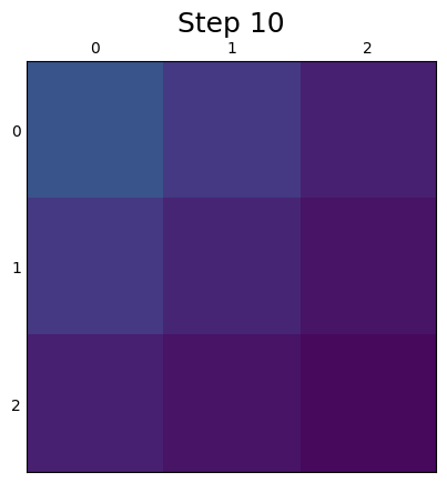

See ex6a.json and ex6a.c for full PopJSON representation and C translation. Use plot_ex6.py to run the model.
Genetic structure and inheritance
We can introduce genetic structure to the spatially-explicit population above by adding just a few more lines of PopJSON. First, we divide the population into immatures and adults. Then, configure the necessary stage transformations (adult emergence and ovipositioning), and finally, set up adult mobility across the spatial scale.
{
    "populations": [
        ["for", "G", 0, 2, ["for", "XY", 0, 63, {
            "id": "immature_[G]_[XY]",
            "name": "Immature stages (combined)",
            "processes": [
                {
                    "id": "immature_dev_[G]_[XY]",
                    "name": "Development time",
                    "arbiter": "ACC_ERLANG",
                    "value": ["pr_stage_duration_mn", "pr_stage_duration_sd"]
                }
            ]
        } ]],
        ["for", "G", 0, 2, ["for", "XY", 0, 63, {
            "id": "adult_[G]_[XY]",
            "name": "Adult females",
            "processes": [
                {
                    "id": "adult_mort_[G]_[XY]",
                    "name": "Adult lifetime",
                    "arbiter": "ACC_ERLANG",
                    "value": ["pr_stage_duration_mn", "pr_stage_duration_sd"]
                }
            ]
        } ]]
    ]
}
In this definition of the populations, we use nested for loops to structure both immatures and adults into 3 genotypes (AA, Aa, and aa) and 64 locations.
{
    "transformations": [
        ["for", "G", 0, 2, ["for", "XY", 0, 63, {
            "id": "emergence_[G]_[XY]",
            "to": "adult_[G]_[XY]",
            "value": "immature_dev_[G]_[XY]"
        } ]],
        ["for", "Ga", 0, 2, ["for", "Gb", 0, 2, ["for", "Gab", 0, 2, ["for", "XY", 0, 63, {
            "id": "ovipos_[Ga]_[Gb]_[Gab]_[XY]",
            "to": "immature_[Gab]_[XY]",
            "value": ["*","pr_F4",["cube","[Ga]","[Gb]","[Gab]"],"adult_[Ga]_[XY]","adult_[Gb]_[XY]"]
        } ]]]]
    ]
}
For each of these sub-groups, we define a transformation from the immature stages to the adult stage. To represent egg laying, we use the nested for loops in the following order: For each location (XY), for each genotype of the progeny (Gab) at that location, and for each genotype of the father (Gb) and mother (Ga) at that location, we extract the fraction of the progeny from the inheritance cube and multiply it with the expected number of eggs (fecundity x males x females). We assume, for simplicity, that the adults are a mixture of males and females and the sex ratio is included in parameter pr_F4.
We define a simple Mendelian inheritance cube for two alleles (A and a) in one locus (for more information about the inheritance cubes, see MGDrivE). Essentially, we assume that when a mother with genotype Aa mates with a father with genotype Aa, their progeny will consist of 25% AA, 50% Aa, and 25% aa individuals.
The cube needs to be supplied as a linear environmental variable (inheritance):
{
    "environ": [
        ["for", "G", 0, 2, {
            "id": "tprob_[G]",
            "name": "Connectivity matrix (fraction of transfer per day)",
            "url": ""
        }],
        {
            "id": "inheritance",
            "name": "The inheritance cube",
            "url": ""
        }
    ]
}
Therefore, the extraction is performed using a simple mapping equation:
{
    "functions": {
        "cube": ["define", ["a","b","c"], ["inheritance", ["+", ["*", "a", 9], ["*", "b", 3], "c"]]]
    }
}
Finally, we define mobility for the three adult genotypes:
{
    "migrations": [
        ["for", "G", 0, 2, {
            "id": "adult_dispersion_[G]",
            "name": "Adult dispersion",
            "prob": "tprob_[G]",
            "target": [["for", "XY", 0, 63, "adult_[G]_[XY]"]]
        }]
    ]
}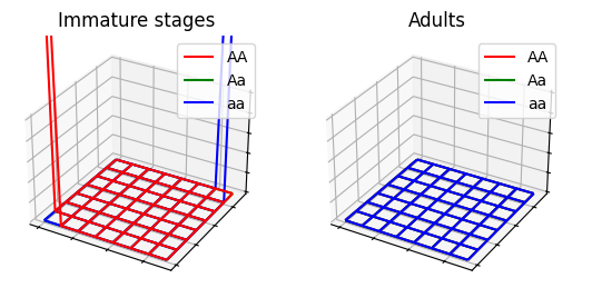
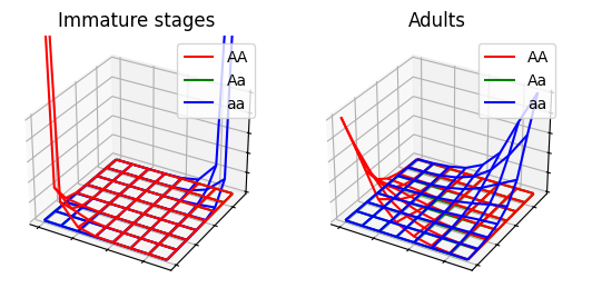
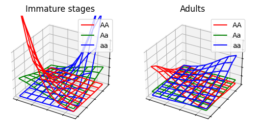
See ex7a.json and ex7a.c for full PopJSON representation and C translation. Use plot_ex7.py to run the model.
Embedding models within models
As of version 1.6.0, this is now possible. As this feature is still under development, it should be used with care and within reasonable limits.
We begin with a simple ODE model describing precipitation-driven breeding site volume.
{
    "reactions": [
        {
            "id": "accumulation",
            "to": {
                "bsvol": 1
            },
            "value": ["*", "alpha", ["prec", "TIME"]]
        },{
            "id": "evaporation",
            "from": {
                "bsvol": 1
            },
            "value": ["*", "beta", "bsvol"]
        }
    ]
}
See ex9.json and ex9.c for full PopJSON representation and C translation. Use plot_ex9.py to run the model.
This should produce something like the following: 
First, we define the outer model - here, a Population model. Using the externals tag, we specify the embedded ODE model by providing the location of the dynamic library (file), along with a brief technical description: the number of state variables (numpop), parameters (numpar), and environmental inputs (numenv).
{
    "model": {
        "title": "Density-dependent population dynamics of Aedes albopictus",
        "type": "Population",
        "url": "https://github.com/kerguler/Population",
        "deterministic": true,
        "parameters": {
            "algorithm": "Population",
            "istep": 0.01
        }
    },
    "externals": [
        {
            "id": "breeding_site",
            "file": "ex9.dylib",
            "numenv": 1,
            "numpar": 2,
            "numpop": 1
        }
    ]
}
We then evaluate this model over a single time step using the evaluate tag, providing the required initial conditions (y0), parameters (pr), and environmental inputs (envir). The results are returned as an array and can be accessed via the specified id.
{
    "evaluate": [
        {
            "id": "bsitevol",
            "value": ["breeding_site", {
                "y0": ["bsvol"],
                "pr": ["bs_alpha","bs_beta"],
                "envir": [["prec", "TIME_1"]]
            }]
        }
    ]
}
The evaluate tag takes precedence and is executed before intermediates, transformations, and transfers. An example of how to reference the output is shown below:
{
    "intermediates": [
        {
            "id": "bsvol",
            "value": ["bsitevol", 0]
        }
    ]
}
It is possible to have evaluate in a process and evaluate the sub-model for each sub-class, maybe using some specific properties of each sub-class.
{
    "processes": [
        {
            "id": "larva_coef",
            "arbiter": "MEMORY",
            "evaluate": [{
                "id": "bsitevol_larva",
                "value": ["breeding_site", {
                    "y0": ["larva_coef"],
                    "pr": ["bs_alpha","bs_beta"],
                    "envir": [["prec", "TIME_1"]]
                }]
            }],
            "value": [["bsitevol_larva", 0]],
            "hazpar": true
        }
    ]
}
Several new features are introduced here, so it is worth examining
this section carefully. The flag "hazpar": true indicates
that the process is evaluated for each sub-class. The process is of type
MEMORY — a new feature — which stores a floating-point
value defined by the value tag. This should be a list
of one element.
In this case, the process evaluates the sub-model
breeding_site using the parameters bs_alpha
and bs_beta, along with the precipitation input for the
current simulation step. The initial condition is taken from the result
of the previous evaluation, which has been stored via the memory
mechanism.
In the second process, shown below, the updated value from this
memory process — already computed at the current step — is used to drive
a larval flushing mechanism. Specifically, larvae are removed when the
breeding site volume exceeds a predefined threshold. This is, of course,
a simplified and hypothetical example intended to illustrate how the
embedded model output can be used within the Population
framework.
{
    "processes": [
        {
            "id": "larva_coef",
            "arbiter": "MEMORY",
            "evaluate": [{
                "id": "bsitevol_larva",
                "value": ["breeding_site", {
                    "y0": ["larva_coef"],
                    "pr": ["bs_alpha","bs_beta"],
                    "envir": [["prec", "TIME_1"]]
                }]
            }],
            "value": [["bsitevol_larva", 0]],
            "hazpar": true
        },{
            "id": "larva_mort",
            "name": "Larva mortality",
            "arbiter": "NOAGE_CONST",
            "intermediates": [{
                "id": "d2m_coef",
                "value": ["?", [">", "larva_coef", "0.75"], "0.5", "0.0"]
            }],
            "value": ["d2m_coef"],
            "hazpar": true
        }
    ]
}
See ex10.json and ex10.c for full PopJSON representation and C translation. Use plot_ex10.py to run the model.
Note the use of intermediates within a process — this is a new feature in version 1.6.0. These intermediates are intended for temporary calculations: they can be useful for structuring expressions but are not retained or reported as outputs. As such, they must be assigned a value before being referenced. Please be reminded that the global intermediates are initialised to 0 by default.
And voilà! 
Operators for equations
| Operator | Parameters | Definition |
|---|---|---|
| min | a,b | Minimum of two numbers |
| max | a,b | Maximum of two numbers |
| abs | a | Absolute value |
| round | a | Rounds to the nearest integer |
| sqrt | a | Square root |
| pow | a,b | Power of a to b |
| exp | a | Exponential function |
| log | a | Natural logarithm |
| log2 | a | Logarithm of a to base 2 |
| log10 | a | Logarithm of a to base 10 |
| indicator | a | Indicator function (boolean to integer) |
| index | a,b | Value of an array at position b (counts from 0) (deprecated) |
| * | … | Multiplication |
| + | … | Addition |
| - | … | Subtraction (in the given order) |
| / | … | Division (in the given order) |
| % | a,b | Modulus operator |
| size | a | Total size of a population (deprecated) |
| count | a,b | Sub-group counts of population a based on a logical check b of sub-group keys |
| poisson | a | Generates a Poisson random number with lambda=a (works only when deterministic:false) |
| binomial | a,b | Generates a Binomial random number with n=a and p=b (works only when deterministic:false) |
| define | a,b | Function definition with parameters a and equation b |
| ? | a,b,c | Condition expression (if a is true, return b, else, return c) |
| && | … | Logical AND |
| || | … | Logical OR |
| ! | a | Logical NOT |
| > | a,b | Logical greater than |
| < | a,b | Logical smaller than |
| >= | a,b | Logical greater than or equal |
| <= | a,b | Logical smaller than or equal |
| == | a,b | Logical equal to |
Examples
- ex1a.json
- ex1b.json
- ex1c.json
- ex1E.json
- ex2a.json
- ex2b.json
- ex3a.json
- ex3b.json
- ex4a.json
- ex5a.json
- ex6a.json
- ex7a.json
- ex8.json
- ex9.json
- ex10.json